5.2. Example 2 - J-band Longslit Point Source - Using the “reduce” command line

In this example, we will reduce the GNIRS J-band longslit observation of a metal-poor M dwarf, using the “reduce” command that is operated directly from the unix shell. Just open a terminal and load the DRAGONS conda environment to get started.

This observation uses the 111 l/mm grating, the short-blue camera, a 0.3 arcsec slit, and is set to a central wavelength of 1.22 ${\mu}$ m. The dither pattern is two consecutive ABBA sequences.

5.2.1. The dataset

If you have not already, download and unpack the tutorial’s data package. Refer to Downloading tutorial datasets for the links and simple instructions.

The dataset specific to this example is described in:

Example 2 - Datasets description

Here is a copy of the table for quick reference.

Science	N20180201S0052-59
Science flats	N20180201S0060-64
Science arcs	N20180201S0065
Telluric	N20180201S0071-74
BPM	bpm_20100716_gnirs_gnirsn_11_full_1amp.fits

5.2.2. Configuring the interactive interface

In ~/.dragons/, add the following to the configuration file dragonsrc:

[interactive]
browser = your_preferred_browser

The [interactive] section defines your preferred browser. DRAGONS will open the interactive tools using that browser. The allowed strings are “safari”, “chrome”, and “firefox”.

5.2.3. Set up the Local Calibration Manager

Important

Remember to set up the calibration service.

Instructions to configure and use the calibration service are found in Setting up the Calibration Service, specifically the these sections: The Configuration File and Usage from the Command Line.

We recommend that you clean up your working directory (playground) and start a fresh calibration database (caldb init -w) when you start a new example.

5.2.4. Create file lists

This data set contains science and calibration frames. For some programs, it could contain different observed targets and different exposure times depending on how you like to organize your raw data.

The DRAGONS data reduction pipeline does not organize the data for you. You have to do it. However, DRAGONS provides tools to help you with that.

The first step is to create input file lists. The tool “dataselect” helps with that. It uses Astrodata tags and descriptors to select the files and send the filenames to a text file that can then be fed to “reduce”. (See the Astrodata User Manual for information about Astrodata and for a list of descriptors.)

First, navigate to the playground directory in the unpacked data package:

cd <path>/gnirsls_tutorial/playground

5.2.4.1. A list for the flats

The GNIRS flats will be stacked together. Therefore it is important to ensure that the flats in the list are compatible with each other. You can use “dataselect” to narrow down the selection as required. Here, we have only the flats that were taken with the science and we do not need extra selection criteria.

dataselect ../playdata/example2/*.fits --tags FLAT -o flats.lis

5.2.4.2. A list for the arcs

The GNIRS longslit arc was obtained at the end of the science observation. Often two are taken. We will use both in this case and stack them later.

dataselect ../playdata/example2/*.fits --tags ARC -o arcs.lis

5.2.4.3. A list for the telluric

DRAGONS does not recognize the telluric star as such. This is because, at Gemini, the observations are taken like science data and the GNIRS headers do not explicitly state that the observation is a telluric standard. In most cases, the observation_class descriptor can be used to differentiate the telluric from the science observations, along with the rejection of the CAL tag to reject flats and arcs.

dataselect ../playdata/example2/*.fits --xtags=CAL --expr='observation_class=="partnerCal"' -o telluric.lis

5.2.4.4. A list for the science observations

The science observations can be selected from the observation class, science, that is how they are differentiated from the telluric standards which are partnerCal.

If we had multiple targets, we would need to split them into separate list. To inspect what we have we can use dataselect and showd together.

dataselect ../playdata/example2/*.fits --expr='observation_class=="science"' | showd -d object

----------------------------------------------------
filename                                      object
----------------------------------------------------
../playdata/example2/N20180201S0052.fits   target_37
../playdata/example2/N20180201S0053.fits   target_37
../playdata/example2/N20180201S0054.fits   target_37
../playdata/example2/N20180201S0055.fits   target_37
../playdata/example2/N20180201S0056.fits   target_37
../playdata/example2/N20180201S0057.fits   target_37
../playdata/example2/N20180201S0058.fits   target_37
../playdata/example2/N20180201S0059.fits   target_37

Here we only have one object from the same sequence. If we had multiple objects we could add the object name in the expression.

dataselect ../playdata/example2/*.fits --expr='observation_class=="science" and object=="target_37"' -o sci.lis

5.2.5. Bad Pixel Mask

Starting with DRAGONS v3.1, the bad pixel masks (BPMs) are handled as calibrations. They are downloadable from the archive instead of being packaged with the software. They are automatically associated like any other calibrations. This means that the user now must download the BPMs along with the other calibrations and add the BPMs to the local calibration manager.

See Get the BPMs in Tips and Tricks to learn about the various ways to get the BPMs from the archive.

To add the static BPM included in the data package to the local calibration database:

caldb add ../playdata/example2/bpm*.fits

5.2.6. Master Flat Field

GNIRS longslit flat fields are normally obtained at night along with the observation sequence to match the telescope and instrument flexure.

The GNIRS longslit flatfield requires only lamp-on flats. Subtracting darks only increases the noise.

The flats will be stacked.

reduce @flats.lis

GNIRS data are affected by a “odd-even” effect where alternate rows in the GNIRS science array have gains that differ by approximately 10 percent. We have added a correction in normalizeFlat that levels off the rows to help with the fit. Here it works well, in some cases you might see a some split when you run normalizeFlat in interactive mode. The objective if you see the split is to get a fit that falls inbetween the two sets of points, with a symmetrical residual fit.

Note that you are not required to run in interactive mode, but you might want to if flat fielding is critical to your program.

reduce @flats.lis -p interactive=True

The interactive tools are introduced in section Interactive tools.

5.2.7. Processed Arc - Wavelength Solution

Obtaining the wavelength solution for GNIRS longslit data can be a complicated topic. The quality of the results and what to use depend greatly on the wavelength regime and the grating.

Our configuration in this example is J-band with a central wavelength of 1.22 ${\mu}$ m, using the 111 l/mm grating. Arcs are available, however, depending on the central wavelength setting, there might be cases where there are too few lines or the coverage is not adequate to get a good solution.

In our current case, the numbers of arcs lines and sky lines are similar. Either solution could work. We will show the result of both. It is up to the user to decide which solution is best for their science.

5.2.7.1. Using the arc lamp

Because the slit length does not cover the whole array, we want to know where the unilluminated areas are located and ignore them when the distortion correction is calculated (along with the wavelength solution). That information is measured during the creation of the flat field and stored in the processed flat. Using the flat is optional but it is recommended. In any case, if a matching flat exists, it will be picked up automatically by the calibration manager.

reduce @arcs.lis -p interactive=True

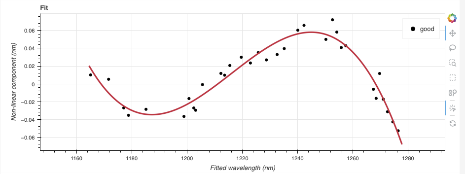
Here, increasing the order to 4 helps to get a tighter fit.

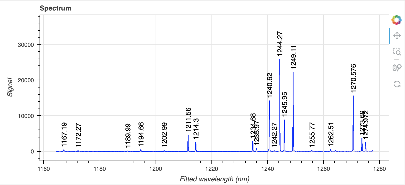
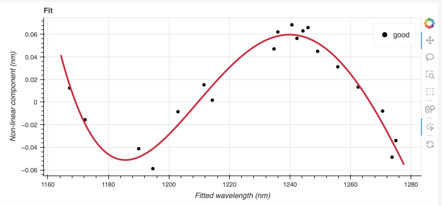
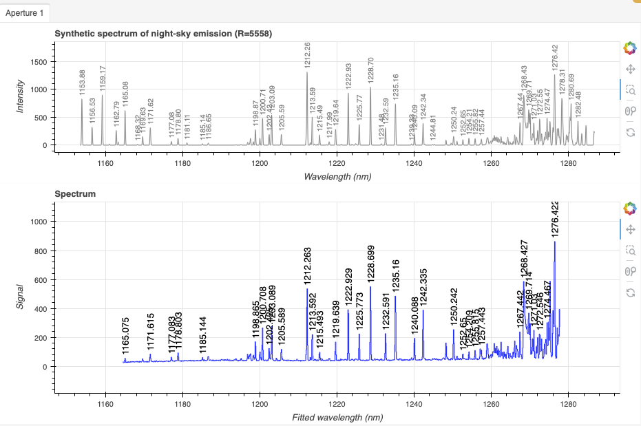
5.2.7.2. Using the sky lines

The spectrum has a number of OH and O₂ sky lines that can be used to create a wavelength solution. The calibration can be done on a single frame or, in case of multiple input frames, the frames will be stacked. It is recommended to use only one frame for a more precise wavelength solution, unless multiple frames are needed to increase the signal-to-noise ratio. Here we will use all the frames in the sci.lis list.

Wavelength calibration from sky lines is better done in interactive mode despite our efforts to automate the process.

To use the sky lines in the science frames instead of the lamp arcs, we invoke the makeWavecalFromSkyEmission recipe.

reduce @sci.lis -r makeWavecalFromSkyEmission -p interactive=True

In this case, using all the frames, we get a good signal to noise and an automatic fit. If you wanted, you could identify more sky lines manually.

Sky lines identification with reference spectrum

Tip

If the sky lines were too weak and no fit were found, a possible solution is to lower the minimum SNR to 5 (down from the default of 10). This setting is in the left control panel. When done, click the the “Reconstruct points” button.

When lowering the SNR, lowering the high and low sigma clipping to 2 will help reject some of the weak blended lines that are more inaccurate.

5.2.7.3. Which solution to use?

Each case will be slightly different. Whether you decide to use the solution from the arc lamp or the sky lines is up to you.

Once you have decided, we recommend that you remove the one you do not want to use from the calibration manager database. Since the _arc file selected will always be the “closest in time” to the science observation, there might be cases where the lamp solution will be picked for the last datasets in the sequence while the sky lines solution will be picked for the first datasets in the sequence.

So pick one, remove the other.

caldb remove N20180201S0065_arc.fits  # remove the lamp solution
... or ...
caldb remove N20180201S0052_arc.fits  # remove the sky line solution

In this tutorial, we remove the lamp solution.

If you wanted to try it anyway for telluric standard reduction or the science reduction, you can force its use with the --user_cal option on the command line, eg --user_cal processed_arc:N20180201S0065_arc.fits.

5.2.8. Telluric Standard

The telluric standard observed after the science observation is “hip 55627”. The spectral type of the star is A0V.

To properly calculate and fit a telluric model to the star, we need to know its effective temperature. To properly scale the sensitivity function (to use the star as a spectrophotometric standard), we need to know the star’s magnitude. Those are inputs to the fitTelluric primitive.

The default effective temperature of 9650 K is typical of an A0V star, which is the most common spectral type used as a telluric standard. Different sources give values between 9500 K and 9750 K and, for example, Eric Mamajek’s list “A Modern Mean Dwarf Stellar Color and Effective Temperature Sequence” (https://www.pas.rochester.edu/~emamajek/EEM_dwarf_UBVIJHK_colors_Teff.txt) quotes the effective temperature of an A0V star as 9700 K. The precise value has only a small effect on the derived sensitivity and even less effect on the telluric correction, so the temperature from any reliable source can be used. Using Simbad, we find that the star has a magnitude of J=9.2.

Instead of typing the values on the command line, we will use a parameter file to store them. In a normal text file (here we name it “hip55627.param”), we write:

-p
fitTelluric:bbtemp=9700
fitTelluric:magnitude='J=9.2'

Then we can call the reduce command with the parameter file. The telluric fitting primitive can be run in interactive mode.

Note that the data are recognized by Astrodata as normal GNIRS longslit science spectra. To calculate the telluric correction, we need to specify the telluric recipe (-r reduceTelluric), otherwise the default science reduction will be run.

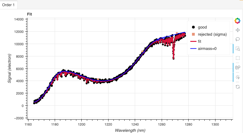
reduce @telluric.lis -r reduceTelluric @hip55627.param -p fitTelluric:interactive=True

Adjusting the order of the spline to 9 leads to more randomized residuals (second panel).

5.2.9. Science Observations

The science target is a low metallicity M-dwarf. The sequence is two ABBA dithered observations. DRAGONS will flat field, wavelength calibrate, subtract the sky, stack the aligned spectra, extract the source, and finally remove telluric features and flux calibrate.

Following the wavelength calibration, the default recipe has an optional step to adjust the wavelength zero point using the sky lines. By default, this step will NOT make any adjustment. We found that in general, the adjustment is so small as being in the noise. If you wish to make an adjustment, or try it out, see Adjusting the Wavelength Zeropoint to learn how.

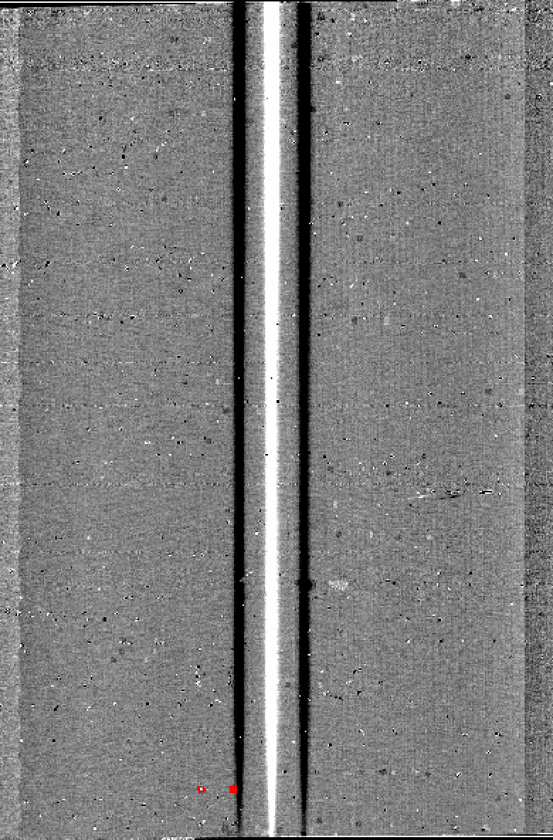
This is what one raw image looks like.

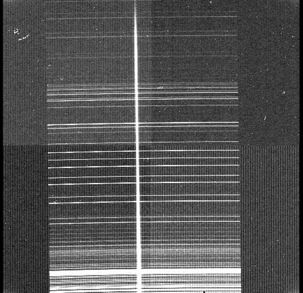
With all the calibrations in the local calibration manager, one only needs to call reduce on the science frames to get an extracted spectrum.

reduce @sci.lis

To run the reduction with all the interactive tools activated, set the interactive parameter to True.

reduce @sci.lis -p interactive=True

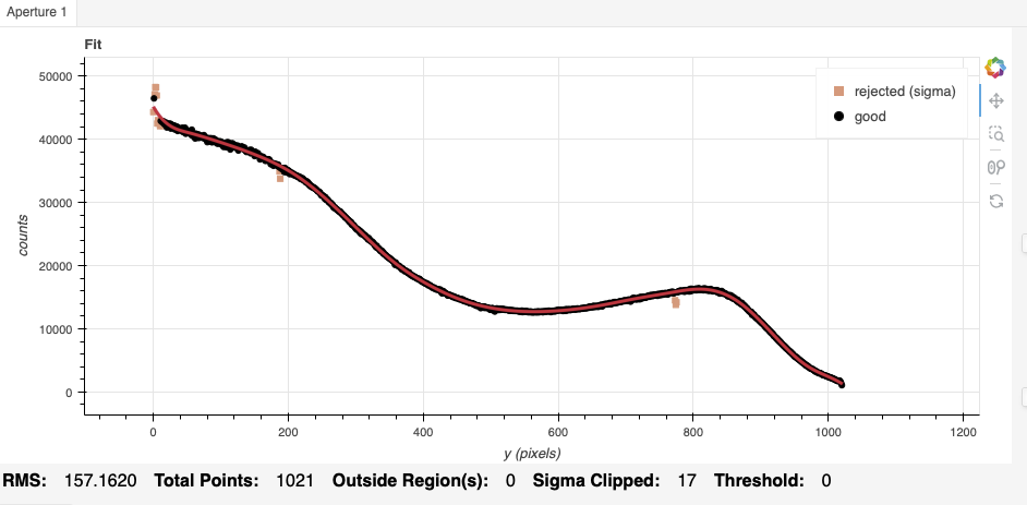
The second aperture detected by findApertures is just a spurious detection. In interactive mode, you can remove it. Or leave, it won’t hurt anything.

The 2D spectrum, without telluric correction and flux calibration, looks like this:

reduce -r display N20180201S0052_2D.fits

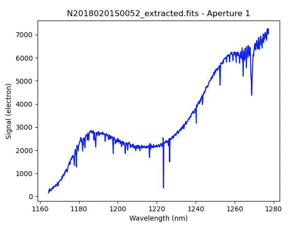
The 1D extracted spectrum before telluric correction or flux calibration, obtained with -p extractSpectra:write_outputs=True, looks like this.

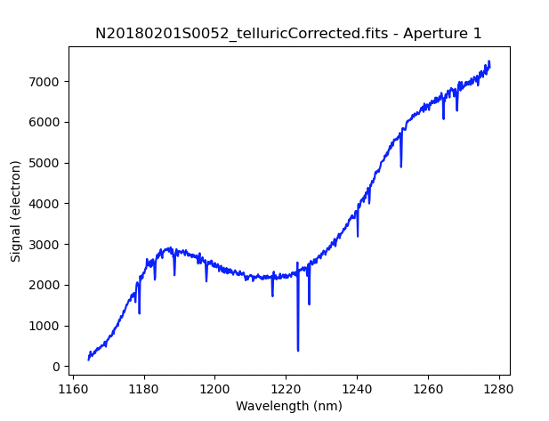
The 1D extracted spectrum after telluric correction but before flux calibration, obtained with -p telluricCorrect:write_outputs=True, looks like this.

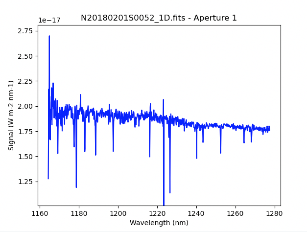
1D extracted spectrum after telluric correction or before flux calibration

And the final spectrum, corrected for telluric features and flux calibrated.

dgsplot N20180201S0052_1D.fits 1

1D extracted spectrum after telluric correction and flux calibration