7.2. Example 4 - K-band 2.33 micron Longslit Point Source (111 l/mm grating) - Using the “reduce” command line

We will reduce the GNIRS K-band longslit observation of HD 179821, likely a yellow hypergiant star, using the “reduce” command that is operated directly from the unix shell. Just open a terminal and load the DRAGONS conda environment to get started.

The observation uses the 111 l/mm grating, the long-blue camera, a 0.3 arcsec slit, and is centered at 2.33 m. The dither pattern is a ABBA sequence.

7.2.1. The dataset

If you have not already, download and unpack the tutorial’s data package. Refer to Downloading tutorial datasets for the links and simple instructions.

The dataset specific to this example is described in:

Example 4 - Datasets description

Here is a copy of the table for quick reference.

Science	N20210407S0173-176
Science flats	N20210407S0177-180
Science arcs	N20210407S0181-182
Telluric	N20210407S0188-191
BPM	bpm_20121101_gnirs_gnirsn_11_full_1amp.fits

7.2.2. Configuring the interactive interface

In ~/.dragons/, add the following to the configuration file dragonsrc:

[interactive]
browser = your_preferred_browser

The [interactive] section defines your preferred browser. DRAGONS will open the interactive tools using that browser. The allowed strings are “safari”, “chrome”, and “firefox”.

7.2.3. Set up the Local Calibration Manager

Important

Remember to set up the calibration service.

Instructions to configure and use the calibration service are found in Setting up the Calibration Service, specifically the these sections: The Configuration File and Usage from the Command Line.

We recommend that you clean up your working directory (playground) and start a fresh calibration database (caldb init -w) when you start a new example.

7.2.4. Create file lists

This data set contains science and calibration frames. For some programs, it could contain different observed targets and different exposure times depending on how you like to organize your raw data.

The DRAGONS data reduction pipeline does not organize the data for you. You have to do it. However, DRAGONS provides tools to help you.

The first step is to create input file lists. The tool “dataselect” helps with that. It uses Astrodata tags and “descriptors” to select the files and send the filenames to a text file that can then be fed to “reduce”. (See the Astrodata User Manual for information about Astrodata and for a list of descriptors.)

First, navigate to the playground directory in the unpacked data package:

cd <path>/gnirsls_tutorial/playground

7.2.4.1. A list for the flats

The GNIRS flats will be stacked together. Therefore it is important to ensure that the flats in the list are compatible with each other. You can use “dataselect” to narrow down the selection as required. Here, we have only the flats that were taken with the science and we do not need extra selection criteria.

dataselect ../playdata/example4/*.fits --tags FLAT -o flats.lis

7.2.4.2. A list for the arcs

The GNIRS longslit arc was obtained at the end of the science observation. Often two are taken. We will use both in this case and stack them later.

dataselect ../playdata/example4/*.fits --tags ARC -o arcs.lis

7.2.4.3. A list for the telluric

DRAGONS does not recognize the telluric star as such. This is because, at Gemini, the observations are taken like science data and the GNIRS headers do not explicitly state that the observation is a telluric standard. For now, the observation_class descriptor can be used to differential the telluric from the science observations, along with the rejection of the CAL tag to reject flats and arcs. The observation_class can be partnerCal or progCal. In this case, it is progCal.

dataselect ../playdata/example4/*.fits --xtags=CAL --expr='observation_class=="progCal"' -o telluric.lis

7.2.4.4. A list for the science observations

The science observations can be selected from the observation class, science, that is how they are differentiated from the telluric standards which are partnerCal or progCal.

If we had multiple targets, we would need to split them into separate lists. To inspect what we have we can use dataselect and showd together.

dataselect ../playdata/example4/*.fits --expr='observation_class=="science"' | showd -d object

----------------------------------------------------
filename                                      object
----------------------------------------------------
../playdata/example4/N20210407S0173.fits   HD 179821
../playdata/example4/N20210407S0174.fits   HD 179821
../playdata/example4/N20210407S0175.fits   HD 179821
../playdata/example4/N20210407S0176.fits   HD 179821

Here we only have one object from the same sequence. If we had multiple objects we could add the object name in the expression.

dataselect ../playdata/example4/*.fits --expr='observation_class=="science" and object=="HD 179821"' -o sci.lis

7.2.5. Bad Pixel Mask

Starting with DRAGONS v3.1, the bad pixel masks (BPMs) are handled as calibrations. They are downloadable from the archive instead of being packaged with the software. They are automatically associated like any other calibrations. This means that the user now must download the BPMs along with the other calibrations and add the BPMs to the local calibration manager.

See Get the BPMs in Tips and Tricks to learn about the various ways to get the BPMs from the archive.

To add the static BPM included in the data package to the local calibration database:

caldb add ../playdata/example4/bpm*.fits

7.2.6. Master Flat Field

GNIRS longslit flat fields are normally obtained at night along with the observation sequence to match the telescope and instrument flexure.

The GNIRS longslit flatfield requires only lamp-on flats. Subtracting darks only increases the noise.

The flats will be stacked.

reduce @flats.lis

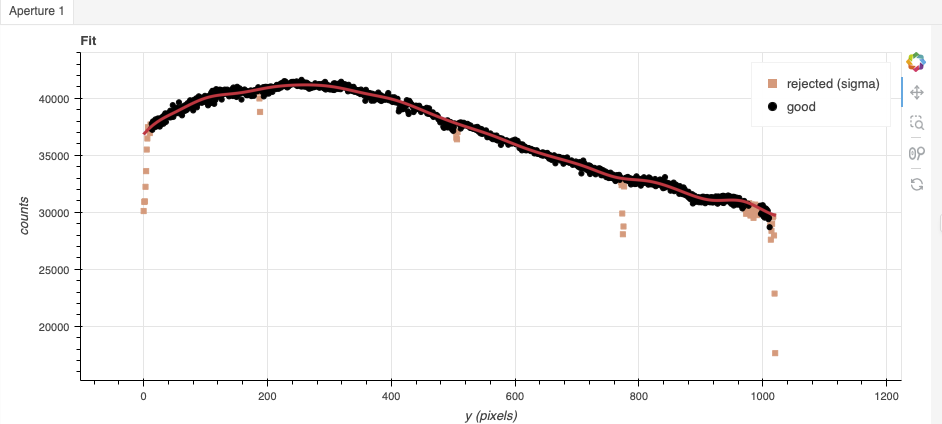
GNIRS data are affected by a “odd-even” effect where alternate rows in the GNIRS science array have gains that differ by approximately 10 percent. We have added a correction in normalizeFlat that levels off the rows to help with the fit. Here it works well, in some cases you might see a some split when you run normalizeFlat in interactive mode. The objective, if you see the split, is to get a fit that falls inbetween the two sets of points, with a symmetrical residual fit.

Note that you are not required to run in interactive mode, but you might want to if flat fielding is critical to your program. In this case, the fit can be improved by activating the sigma clipping with one iteration, setting the low sigma to 2 instead of 3, and setting the “grow” parameter to 2.

reduce @flats.lis -p interactive=True

The interactive tools are introduced in section Interactive tools.

7.2.7. Processed Arc - Wavelength Solution

Obtaining the wavelength solution for GNIRS longslit data can be a complicated topic. The quality of the results and what to use depends greatly on the wavelength regime and the grating.

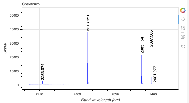
Our observations are K-band at a central wavelength of 2.33 m using the 111/mm grating. In that regime, the arc lamp observation contains very few lines, five in this case which fortunately are correctly identified. The number of lines can be as low as 2 or 3 in redder settings. It is impossible to have an accurate solution from the arc alone.

The other difficulty is that the OH and O₂ lines are absent in that regime. There are no emission lines. There are however a large number of telluric absorption lines in the target’s spectrum.

Therefore, we will use the arc lamp solution as the starting point for the calculation of the solution derived from the telluric absorption lines.

7.2.7.1. The arc lamp solution

Because the slit length does not cover the whole array, we want to know where the unilluminated areas are located and ignore them when the distortion correction is calculated (along with the wavelength solution). That information is measured during the creation of the flat field and stored in the processed flat. Right now, the association rules do not automatically associate flats to arcs, therefore we need to specify the processed flat on the command line. Using the flat is optional but it is recommended when using an arc lamp.

Turning on the interactive mode is recommended. The lines are correctly identified in this case, but at redder settings it is not always the case. Plots of the arc lamps with wavelength labels can be found here:

https://www.gemini.edu/instrumentation/gnirs/calibrations#Arc

The arc we are processing was taken with the Argon lamp.

Once the coarse arc is calculated it will automatically be added to the calibration database. We do not want that arc to ever be used during the reduction of the science data. So we immediately remove it from the database. We will feed it to the next step, the only one that needs it, manually.

reduce @arcs.lis -p interactive=True
caldb remove N20210407S0181_arc.fits

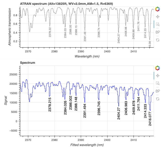
7.2.7.2. The telluric absorption lines solution

Because only the telluric absorption lines provide a good spectral coverage in this configuration, we are forced to use them.

To use the telluric absorption lines in the science frames instead of the lamp arcs, we invoke the makeWavecalFromSkyAbsorption recipe. It will get the arc lamp solution from the calibration manager automatically and use it as an initial approximation.

It is strongly recommended to use the interactive mode to visually confirm that lines have been properly identified and if not manually identify the lines.

reduce @sci.lis -r makeWavecalFromSkyAbsorption --user_cal processed_arc:N20210407S0181_arc.fits -p  interactive=True

In this case, indeed, there is a discrepancy.

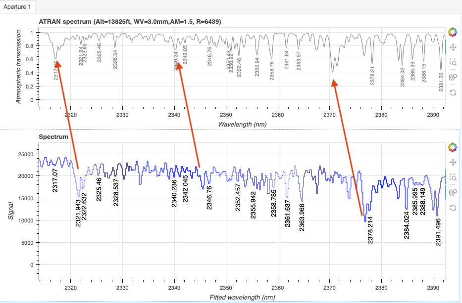
The first step to correct the situation is to clear the lines and then use “i” to identify lines correctly with the help of the top plot. After a few have been identified across the entire spectrum, click “Identify Lines” to fill in more lines automatically.

7.2.8. Telluric Standard

The telluric standard observed before the science observation is “hip 92386”. The spectral type of the star is A1IV.

To properly calculate and fit a telluric model to the star, we need to know its effective temperature. To properly scale the sensitivity function (to use the star as a spectrophotometric standard), we need to know the star’s magnitude. Those are inputs to the fitTelluric primitive.

From Eric Mamajek’s list “A Modern Mean Dwarf Stellar Color and Effective Temperature Sequence” (https://www.pas.rochester.edu/~emamajek/EEM_dwarf_UBVIJHK_colors_Teff.txt) we find that the effective temperature of an A1V star is about 9300 K. Prieto & del Burgo, 2016, MNRAS, 455, 3864, finds an effective temperature of 8894 K for HIP 92386 (HD 174240). The exact temperature should not matter all that much. We are using the Prieto & del Burgo value here. Using Simbad, we find that the star has a magnitude of K=6.040.

Instead of typing the values on the command line, we will use a parameter file to store them. In a normal text file (here we name it “hip92386.param”), we write:

-p
fitTelluric:bbtemp=8894
fitTelluric:magnitude='K=6.040'

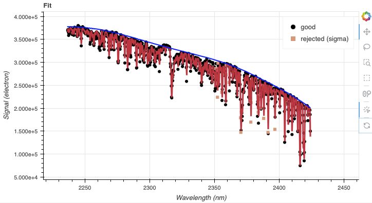
Then we can call the reduce command with the parameter file. The telluric fitting primitive can be run in interactive mode.

Note that the data are recognized by Astrodata as normal GNIRS longslit science spectra. To calculate the telluric correction, we need to specify the telluric recipe (-r reduceTelluric), otherwise the default science reduction will be run.

reduce @telluric.lis -r reduceTelluric @hip92386.param -p interactive=True

In the top plot the blue line represents the continuum and should “envelop” the spectrum (black dots are the data, red line is the telluric model). If the blue line crosses in the middle of the data, for example, this is a sign that the wavelength calibration is not correct. Go back and try to fix the wavelength solution.

Here it all looks good.

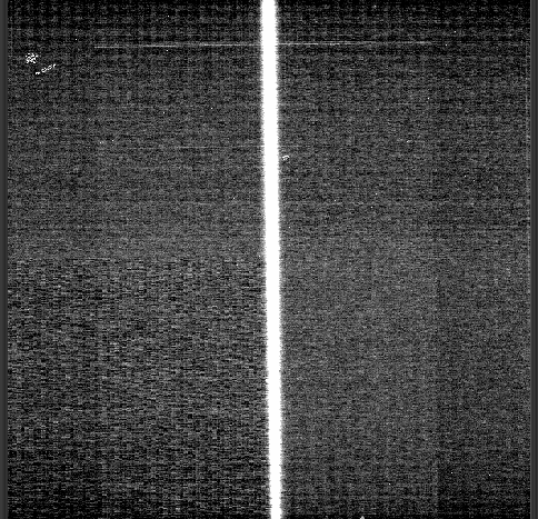
7.2.9. Science Observations

The science target is HD 179821. It is believed to be either a post-asymtotic giant star or a yellow hypergiant. The sequence is one ABBA dithered observations. DRAGONS will flat field, wavelength calibrate, subtract the sky, stack the aligned spectra, extract the source, and finally remove telluric features and flux calibrate.

This is what one raw image looks like.

With all the calibrations in the local calibration manager, one only needs to call reduce on the science frames to get an extracted spectrum.

reduce @sci.lis

To run the reduction with all the interactive tools activated, set the interactive parameter to True.

reduce @sci.lis -p interactive=True

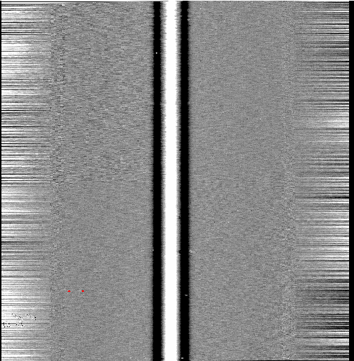
The 2D spectrum, without telluric correction and flux calibration, with blue wavelengths at the bottom and the red-end at the top, looks like this:

reduce -r display N20210407S0173_2D.fits

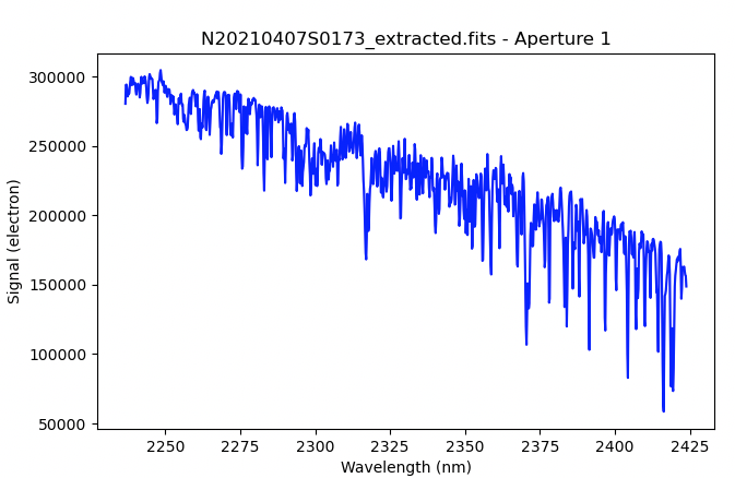
The 1D extracted spectrum before telluric correction or flux calibration, obtained with -p extractSpectra:write_outputs=True, looks like this.

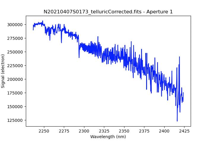
The 1D extracted spectrum after telluric correction but before flux calibration, obtained with -p telluricCorrect:write_outputs=True, looks like this.

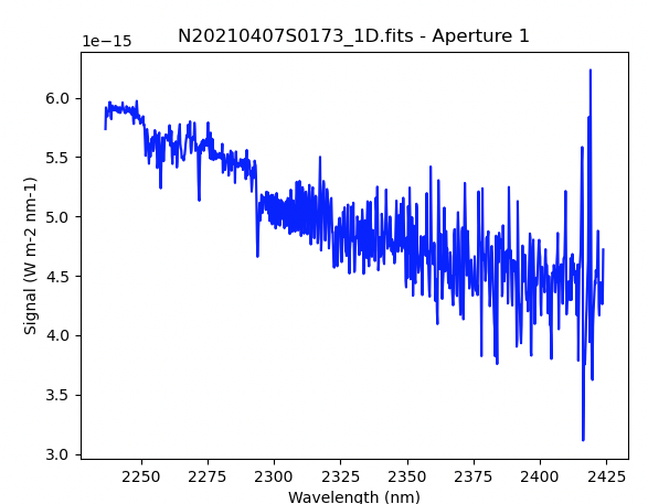
And the final spectrum, corrected for telluric features and flux calibrated.

dgsplot N20210407S0173_1D.fits 1