4.2. Example 1 - K-band Longslit Point Source - Using the “reduce” command line

In this example, we will reduce the GNIRS K-band longslit observation of “SDSSJ162449.00+321702.0”, a white dwarf with an M dwarf companion, using the “reduce” command that is operated directly from the unix shell. Just open a terminal and load the DRAGONS conda environment to get started.

This observation uses the 32 l/mm grating, the short-blue camera, a 0.3 arcsec slit, and is set to a central wavelength of 2.2 m. The dither pattern is the standard ABBA.

4.2.1. The dataset

If you have not already, download and unpack the tutorial’s data package. Refer to Downloading tutorial datasets for the links and simple instructions.

The dataset specific to this example is described in:

Example 1 - Datasets description

Here is a copy of the table for quick reference.

Science	N20170609S0127-130
Science flats	N20170609S0131-135
Science arcs	N20170609S0136
Telluric	N20170609S0118-121
BPM	bpm_20100716_gnirs_gnirsn_11_full_1amp.fits

4.2.2. Configuring the interactive interface

In ~/.dragons/, add the following to the configuration file dragonsrc:

[interactive]
browser = your_preferred_browser

The [interactive] section defines your preferred browser. DRAGONS will open the interactive tools using that browser. The allowed strings are “safari”, “chrome”, and “firefox”.

4.2.3. Set up the Local Calibration Manager

Important

Remember to set up the calibration service.

Instructions to configure and use the calibration service are found in Setting up the Calibration Service, specifically the these sections: The Configuration File and Usage from the Command Line.

We recommend that you clean up your working directory (playground) and start a fresh calibration database (caldb init -w) when you start a new example.

4.2.4. Create file lists

This data set contains science and calibration frames. For some programs, it could contain different observed targets and different exposure times depending on how you like to organize your raw data.

The DRAGONS data reduction pipeline does not organize the data for you. You have to do it. However, DRAGONS provides tools to help you with that.

The first step is to create input file lists. The tool “dataselect” helps. It uses Astrodata tags and descriptors to select the files and send the filenames to a text file that can then be fed to “reduce”. (See the Astrodata User Manual for information about Astrodata and for a list of descriptors.)

First, navigate to the playground directory in the unpacked data package:

cd <path>/gnirsls_tutorial/playground

4.2.4.1. A list for the flats

The GNIRS flats will be stacked together. Therefore it is important to ensure that the flats in the list are compatible with each other. You can use “dataselect” to narrow down the selection as required. Here, we have only the flats that were taken with the science and we do not need extra selection criteria.

dataselect ../playdata/example1/*.fits --tags FLAT -o flats.lis

4.2.4.2. A list for the arcs

The GNIRS longslit arc were obtained at the end of the science observation. Often two are taken. We will use both in this example and stack them later.

dataselect ../playdata/example1/*.fits --tags ARC -o arcs.lis

4.2.4.3. A list for the telluric

DRAGONS does not recognize the telluric star as such. This is because, at Gemini, the observations are taken like science data and the GNIRS headers do not explicitly state that the observation is a telluric standard. In most cases, the observation_class descriptor can be used to differentiate the telluric from the science observations, along with the rejection of the CAL tag to reject flats and arcs.

dataselect ../playdata/example1/*.fits --xtags=CAL --expr='observation_class=="partnerCal"' -o telluric.lis

4.2.4.4. A list for the science observations

The science observations can be selected from the “observation class” science. This is how they are differentiated from the telluric standards which are set to partnerCal.

If we had multiple targets, we would need to split them into separate lists. To inspect what we have we can use dataselect and showd together.

dataselect ../playdata/example1/*.fits --expr='observation_class=="science"' | showd -d object

------------------------------------------------------------------
filename                                                    object
------------------------------------------------------------------
../playdata/example1/N20170609S0127.fits   SDSSJ162449.00+321702.0
../playdata/example1/N20170609S0128.fits   SDSSJ162449.00+321702.0
../playdata/example1/N20170609S0129.fits   SDSSJ162449.00+321702.0
../playdata/example1/N20170609S0130.fits   SDSSJ162449.00+321702.0

Here we only have one object from the same sequence. If we had multiple objects we could add the object name in the expression.

dataselect ../playdata/example1/*.fits --expr='observation_class=="science" and object=="SDSSJ162449.00+321702.0"' -o sci.lis

4.2.5. Bad Pixel Mask

Starting with DRAGONS v3.1, the bad pixel masks (BPMs) are handled as calibrations. They are downloadable from the archive instead of being packaged with the software. They are automatically associated like any other calibrations. This means that the user now must download the BPMs along with the other calibrations and add the BPMs to the local calibration manager.

See Get the BPMs in Tips and Tricks to learn about the various ways to get the BPMs from the archive.

To add the static BPM included in the data package to the local calibration database:

caldb add ../playdata/example1/bpm*.fits

4.2.6. Master Flat Field

GNIRS longslit flat fields are normally obtained at night along with the observation sequence to match the telescope and instrument flexure.

The GNIRS longslit flatfield requires only lamp-on flats. Subtracting darks only increases the noise.

The flats will be stacked.

reduce @flats.lis

GNIRS data are affected by a “odd-even” effect where alternate rows in the GNIRS science array have gains that differ by approximately 10 percent. We have added a correction in normalizeFlat that levels off the rows to help with the fit. Here it works well, in some cases you might see a some split when you run normalizeFlat in interactive mode. The objective, if you see the split, is to get a fit that falls inbetween the two sets of points, with a symmetrical residual fit.

Note that you are not required to run in interactive mode, but you might want to if flat fielding is critical to your program. For example, in this case adjusting the order to 30 significantly improves the fit.

reduce @flats.lis -p interactive=True

The interactive tools are introduced in section Interactive tools.

4.2.7. Processed Arc - Wavelength Solution

Obtaining the wavelength solution for GNIRS longslit data can be a complicated topic. The quality of the results and what to use depend greatly on the wavelength regime and the grating.

Our configuration in this example is K-band with a central wavelength less then 2.3 m, using the 32 l/mm grating. It is expected that the GCAL arc lamp will have a sufficient number of lines available. This is the simplest case. (See Wavelength Calibration Guide for GNIRS LS.)

Because the slit length does not cover the whole array, we want to know where the unilluminated areas are located and ignore them when the distortion correction is calculated (along with the wavelength solution). That information is measured during the creation of the flat field and stored in the processed flat. Using the flat is optional but it is recommended. In any case, if a matching flat exists, it will be picked up automatically by the calibration manager.

reduce @arcs.lis

The primitive determineWavelengthSolution, used in the recipe, has an interactive mode. To activate the interactive mode:

reduce @arcs.lis -p interactive=True

The interactive tools are introduced in section Interactive tools.

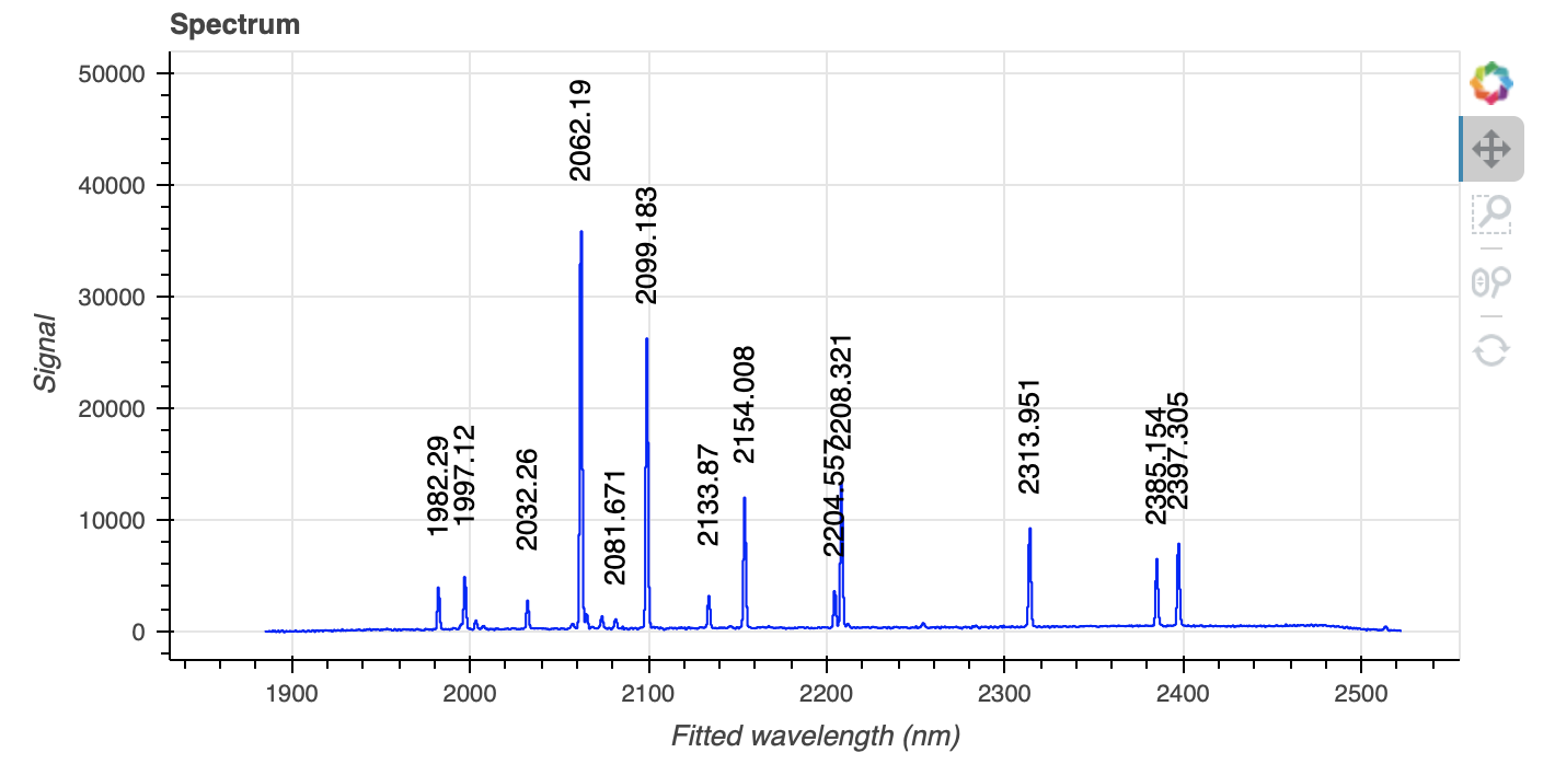
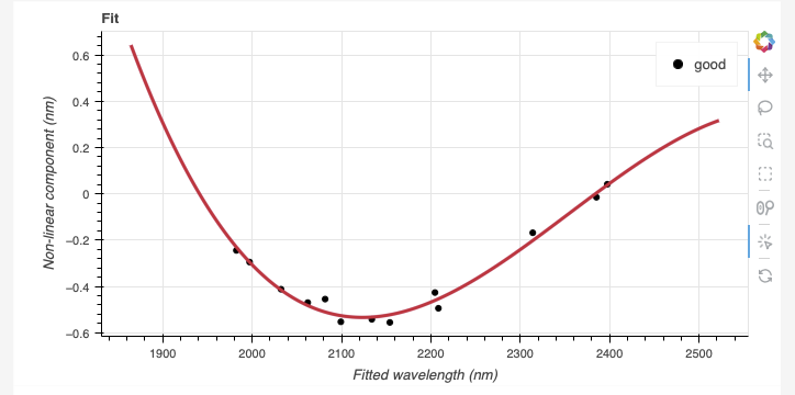
We can see from the interactive tool plot that the wavelength solution has reasonable line coverage between 1.98 and 2.4 m.

We will see later that the final science spectrum goes about 0.1 m beyond the coverage. The solution in the outer area is unconstrained. If the lines of scientific interest are beyond the line list range and wavelength accuracy is very important, using sky lines, if strong enough in the science spectrum, might be a better solution. (Refer to this example.)

4.2.8. Telluric Standard

The telluric standard observed before the science observation is “hip 78649”. The spectral type of the star is A2.5IV.

To properly calculate and fit a telluric model to the star, we need to know its effective temperature. To properly scale the sensitivity function (to use the star as a spectrophotometric standard), we need to know the star’s magnitude. Those are inputs to the fitTelluric primitive.

From Boehm-Vitense, E. 1982 ApJ 255, 191 “Effective temperatures of A and F stars”., Table 2, we find that the effective temperature of an A2.5IV star is about 8150 K. Using Simbad, we find that the star has a magnitude of K=3.925.

Instead of typing the values on the command line, we will use a parameter file to store them. In a normal text file (here we name it “hip78649.param”), we write:

-p
fitTelluric:bbtemp=8150
fitTelluric:magnitude='K=3.925'

Then we can call the reduce command with the parameter file. The telluric fitting primitive can be run in interactive mode.

Note that the data are recognized by Astrodata as normal GNIRS longslit science spectra. To calculate the telluric correction, we need to specify the telluric recipe (-r reduceTelluric), otherwise the default science reduction will be run.

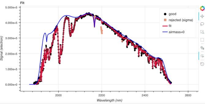
reduce @telluric.lis -r reduceTelluric @hip78649.param -p fitTelluric:interactive=True

Using a spline3 of order 10 leads to a fit that better follows the continuum without being too wavy. The fit might look a bit high in the blue but remember that this is a region where the telluric absorption becomes important.

4.2.9. Science Observations

The science target is a white dwarf with an M dwarf companion. The sequence is one ABBA dither pattern. DRAGONS will flatfield, wavelength calibrate, subtract the sky, stack the aligned spectra, extract the source, and finally remove telluric features and flux calibrate.

Following the wavelength calibration, the default recipe has an optional step to adjust the wavelength zero point using the sky lines. By default, this step will NOT make any adjustment. We found that in general, the adjustment is so small as being in the noise. If you wish to make an adjustment, or try it out, see Adjusting the Wavelength Zeropoint to learn how.

For this dataset, the automatic wavelength zero point algorithm would find a shift of 0.1461 pixels (-0.09408 nm), so not really significant. This is typical and why the default is set to do nothing.

Note

In this observation, there is only one real source to extract. If there were multiple sources in the slit, regardless of whether they are of interest to the program or not, DRAGONS will locate them, trace them, and extract them automatically. Each extracted spectrum is stored in an individual extension in the output multi-extension FITS file.

The automatic source detection in this case does find one extra spurious sources at the extreme left edge of the cross-section. It is not a real source. Just ignore it or remove it in interactive mode.

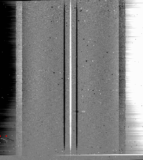
This is what one raw image looks like.

With all the calibrations in the local calibration manager, one only needs to call reduce on the science frames to get an extracted spectrum.

reduce @sci.lis

To run the reduction with all the interactive tools activated, set the interactive parameter to True.

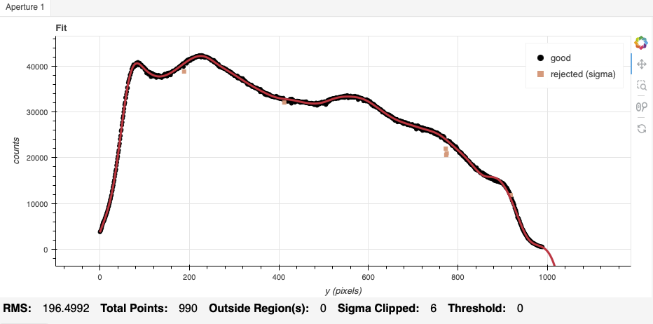
The primitive findApertures finds the source automatically. If it were to find spurious sources, or sources you are simply not interested in, you can remove them by pointing the cursor on them and by pressing d.

It does not make a big difference in this case but at the fitTelluric step we can adjust the offset to 0.1 to better remove the telluric features.

reduce @sci.lis -p interactive=True

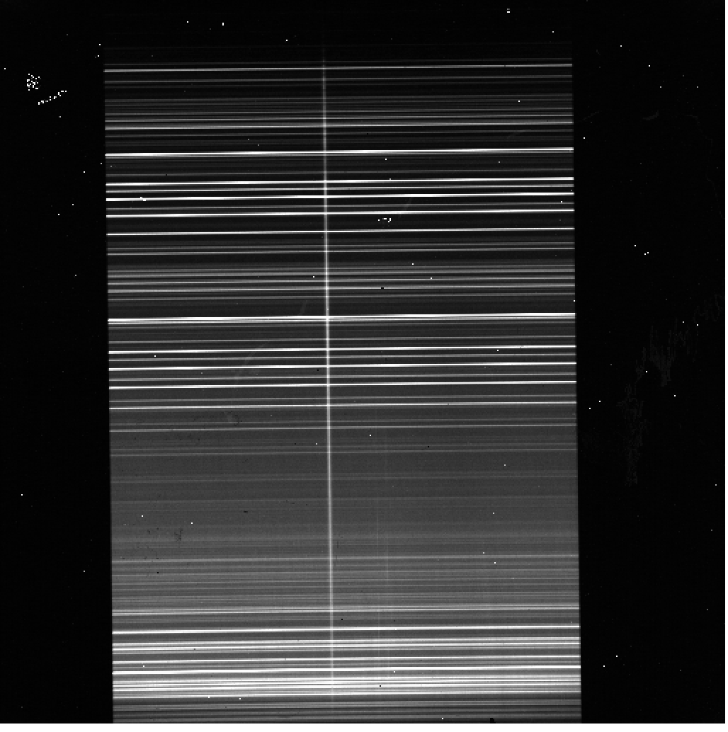
The 2D spectrum before extraction looks like this, with blue wavelengths at the bottom and the red-end at the top.

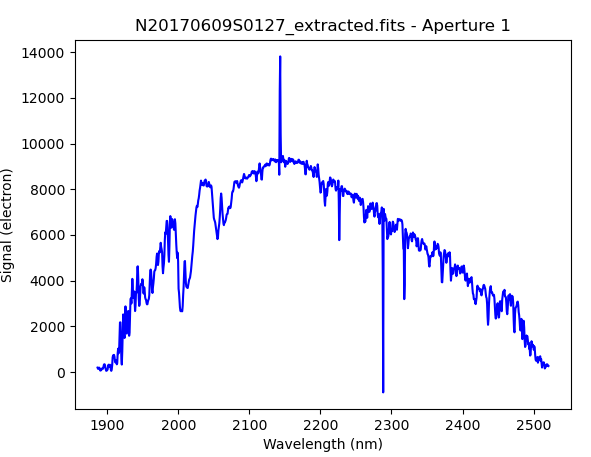
The 1D extracted spectrum before telluric correction or flux calibration, obtained with -p extractSpectra:write_outputs=True, looks like this.

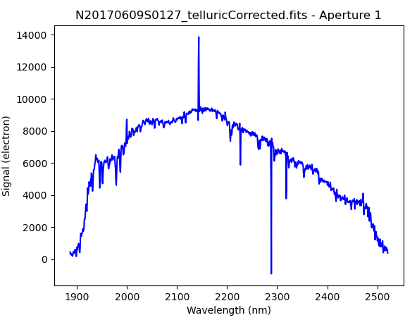
The 1D extracted spectrum after telluric correction but before flux calibration, obtained with -p telluricCorrect:write_outputs=True, looks like this.

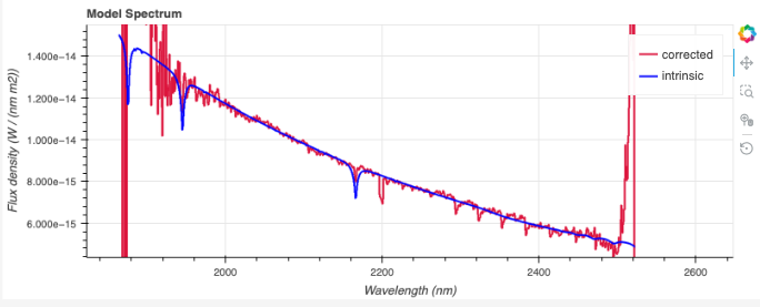
And the final spectrum, corrected for telluric features and flux calibrated.

dgsplot N20170609S0127_1D.fits 1

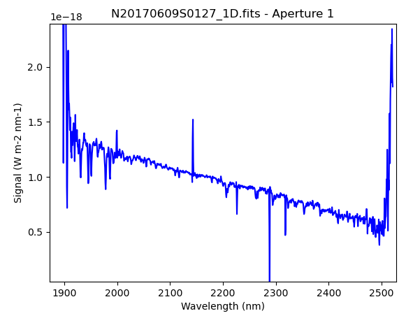
Because of the low signal at the edges, it is not unusual for the flux calibration to diverge at the extremities; the function is simply not well constrained there.